 Michael Crown
data scientist
Marketing Campaign Analysis
Inferring the effects of marketing channel expenditures and gender targeting on unit sales
Executive Summary
This report summarizes the analysis and modeling results of a study to infer the effects of per-channel marketing expenditures on unit sales, with and without the condition of gender targeting. The channels used in the analysis are Adsense display ads, Pinterest promoted pins, and Facebook news feed ads.
Analysis: Methods of analysis include multiple linear regression, t-tests, F-tests, confidence intervals, and cross-correlation. Primary results and figures are in the Results section, and all figures, tables and calculations can be found in the appendix.
Results and Conclusions: In the context of this study, results show that the best performing channel (without considering gender) is Adsense, and the weakest performer is Pinterest. Men are most responsive to Adsense, and are generally unresponsive to promoted pins. Women respond well to both Facebook and Pinterest, and less to Adsense. Cross-correlation shows that the expected time to conversion is one week.
This study concludes that the marketing budget can be allocated more effectively, especially for Adsense and Pinterest campaigns.
Recommendations:
- For male targeting, significantly decrease spending on Pinterest, and increase on Adsense.
- For female targeting, Increase spending on Facebook and Pinterest, and decrease on Adsense.
Limitations: There are many lurking variables in this study that can affect conversion rates for advertisements. A major subset of these fall under conversion tracking: there is no attribution, contextual data, or information about ad content for various campaigns.
INTRODUCTION
This report summarizes the primary analysis and statistical modeling results of a study involving 104 weeks of online marketing campaigns. The primary goal of this analysis is to use multiple regression to infer the effects of marketing expenditures on unit sales across three marketing channels, both with and without the condition of gender targeting. The secondary goal is to estimate the expected time to conversion using cross-correlation.
Two related datasets are used: The first contains week number, weekly spending for three different marketing channels, and the gender targeted in each campaign. The second contains week number and weekly unit sales (the response variable).
QUESTIONS
The questions that motivated this study are:
-
Primary questions:
-
Is there a relationship between marketing channel spending and sales?
- Is at least one of the channels useful in predicting sales?
- Do all or only subset of channels have an effect?
- How well do the models fit the data?
-
What is the expected time to conversion following a campaign?
- Time measured in weeks.
Secondary questions:
- By what magnitude does each channel affect sales?
- Which channels have the most positive effects?
- How accurate are the parameter estimates?
- How does gender affect sales? (overall and per channel)
- Is the true relationship linear?
DATA
The dataset for this project is comprised of two tables (dset1 and dset2) in CSV format, both from a 104 week sample. The first (dset1) has five columns:
- week: the week number
- ads: dollars spend on the Adsense channel
- pin: dollars spent on Pinterest channel
- fb: dollars spent on Facebook channel
- gender: the gender targeted
The second table (dset2) has two columns: week and units_sold (number of units sold that week), and 104 rows — one for each week of unit sales. There are no dates specified, only week number.
ANALYSIS
Preprocessing
Before modeling, the data needed to be in a merged form that allows creation of gender-specific and gender-neutral models. To combine the sets, the spending and gender columns needed to be merged with unit sales according to week number. This merge was done with a simple inner join using the week number as the key, resulting in a single array with 208 rows and six columns (see table 1). This array was name dset and served as a master set for creating the ones to be used in the actual modeling process.
| week | ads | pin | fb | gender | units_sold | |
|---|---|---|---|---|---|---|
| 0 | 1.0 | 11.89 | 70.77 | 259.24 | 0.0 | 119.0 |
| 1 | 1.0 | 128.72 | 243.59 | 19.99 | 1.0 | 119.0 |
| 2 | 2.0 | 137.10 | 170.12 | 48.96 | 0.0 | 112.0 |
| 3 | 2.0 | 17.52 | 136.84 | 379.36 | 1.0 | 112.0 |
| 4 | 3.0 | 260.47 | 143.52 | 276.07 | 0.0 | 133.0 |
The second step was to create a gender-neutral data frame (dfn) with rows of the same week number summed for weekly total spending. This was achieved by grouping the data by week and using summation as the aggregate function, then dropping the gender column. This left the unit sales for every week doubled — a problem that was corrected by dividing all unit_sales values by two.
Before creating the gender-specific sets, cross-correlation was performed on dfn, which is described in the next section, where construction of gendered sets is described.
Exploratory Analysis
Because least squares regression requires statistical independence between predictors, this condition was verified by computing the Pearson correlation coefficient on all predictors (see figure 1). Cross-correlation was performed on unit sales against each of the channels in dfn using using the signal correlation function available in the Python SciPy package. The results showed that correlation was highest for all channels at the -1 lag, which indicates a one week time to conversion. The plotted results of the cross-correlations are below.
Because the cross-correlations show a lag of one week, dfn units_sold were shifted one week to account for the offset. The first step in creating the male and female sets (dfm and dff, respectively) was to create a copy of dset with units_sold shifted up by two weeks (there are two entries per week number). The second step was to filter this set by gender, setting dfm and dff equal to their respective filtered results, and dropping the gender column. The indices on dfm and dff were reset to generic row numbers.
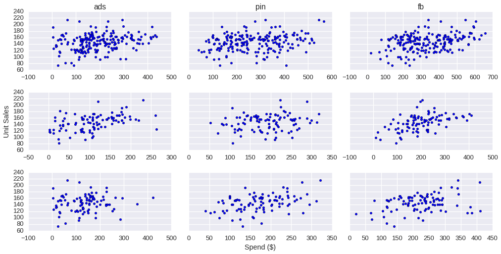
The following scatter plots were produced to gain some visual insight into the relationship between unit sales and each channel, for gender-neutral and gender-specific:
Modeling
A total of 12 models were fitted to the data — four for each of dfm, dff, and dfn: three bivariate models (one for each channel) and one multivariate model using all channels. These were fitted using an ordinary least squares regression algorithm I wrote (found here).
The models output descriptive statistics (see Evaluation) and the estimated parameters bi. The model parameters are the values of interest for answering the first question posed in this study. The estimates for the multivariate models are below.
| Neutral | Male | Female | |
|---|---|---|---|
| b0 | -2.862018 | 91.366817 | 78.718772 |
| b1 | 0.143175 | 0.172782 | 0.041876 |
| b2 | 0.115655 | 0.045164 | 0.188009 |
| b3 | 0.168091 | 0.134592 | 0.128299 |
The b0 value indicates the expected baseline sales with no money spent on advertising, and the values b1-b3 indicate the expected number of unit sales for every dollar spent on a specific channel. As an example, b1 = 0.17 means that a spend of $100 on Adsense in the gender-neutral model is expected to generate sales of 17 units, independent of other channels.
Evaluation
To evaluate the the multivariate models, ANOVA with unconstrained and incremental F-tests were used, and the bivariate models were evaluated using t-tests. The fits of all models were measured using R2 and adjusted R2. The results of the unconstrained F-tests are in the tables below.
| SS | DF | MS | F | p-value | R2 | R2adj | |
|---|---|---|---|---|---|---|---|
| Regression | 53677.99 | 3.0 | 17892.66 | 141.90 | 2.22e-16 | 0.81 | 0.81 |
| Error | 12483.47 | 99.0 | 126.10 | - | - | - | - |
| Total | 66161.46 | 102.0 | 648.64 | - | - | - | - |
| SS | DF | MS | F | p-value | R2 | R2adj | |
|---|---|---|---|---|---|---|---|
| Regression | 25979.75 | 3.0 | 8659.92 | 24.62 | 1.75e-11 | 0.45 | 0.43 |
| Error | 32356.49 | 92.0 | 351.70 | - | - | - | - |
| Total | 58336.24 | 95.0 | 614.07 | - | - | - | - |
| SS | DF | MS | F | p-value | R2 | R2adj | |
|---|---|---|---|---|---|---|---|
| Regresion | 20147.50 | 3.0 | 6715.83 | 14.40 | 1.94e-07 | 0.32 | 0.30 |
| Error | 41983.90 | 90.0 | 466.49 | - | - | - | - |
| Total | 62131.40 | 93.0 | 668.08 | - | - | - | - |
The F-tests were two-sided hypothesis tests of the form:
H0: β1 = β2 = β3 = 0
HA: At least one βi ≠ 0
Where βi are the true parameters. In other words, test the null hypothesis (H0) that there is no relationship between the amounts spent on any of the marketing channels and unit sales. The alternative hypothesis (HA) is that there is a relationship between the amount spent on at least one of the marketing channels and unit sales.
The incremental F-tests were similar, but they tested multivariate models excluding each of the channels, one at a time. This served to estimate the impact of each channel on the complete multivariate models, and determine if any were unimportant. The outcome of the incremental tests are discussed in the results section. Each incremental model kept two of the channels, and tests with only one channel were done in the bivariate models using t-tests. The pairs tested were therefore {(ads, pin), (ads, fb), (pin, fb)}. Using ANOVA results, 95% confidence intervals were constructed for the three multivariate models (see Results).
RESULTS
The estimated parameters for the multivariate models give the following equations for the three models, rounded to three decimal places:
ŷn = -2.862 + 0.143 xads + 0.116 xpin + 0.168 xfb
ŷm = 91.367 + 0.173 xads + 0.045 xpin + 0.135 xfb
ŷf = 78.719 + 0.042 xads + 0.188 xpin + 0.128 xfb
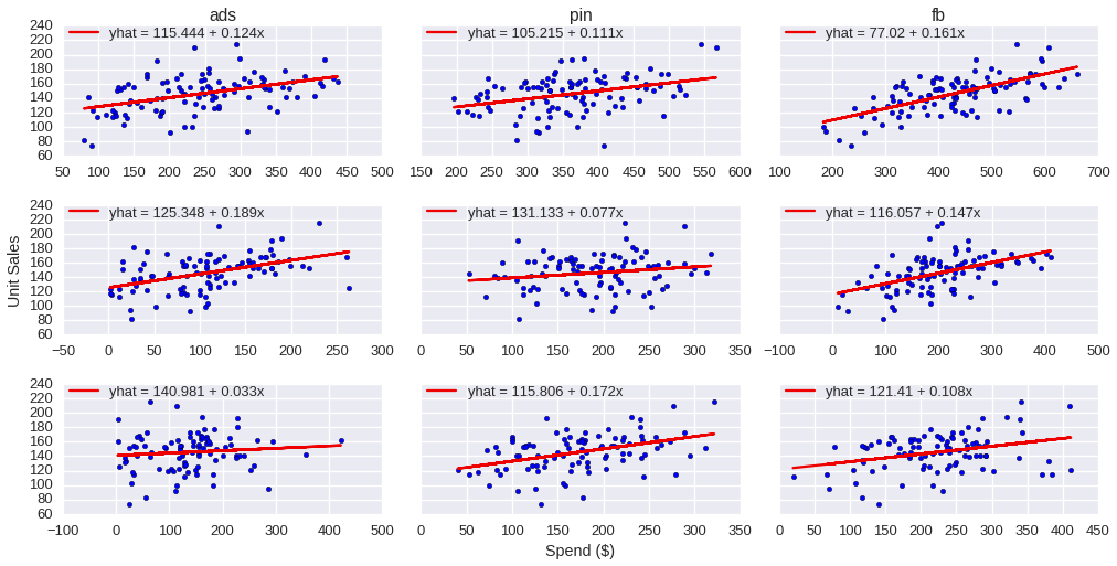
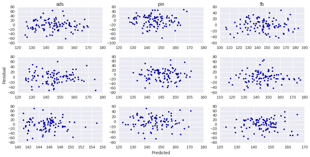
The ŷ values are the estimated number of units sold in response to spending on the three channels, xads, xpin, and xfb in each model. These equations produce hyperplanes that cannot be graphed, but the lines of best fit from the bivariate models are graphed over the scatter plots from figure 3, and their equations are displayed in the legends:
As was seen in tables 3-5, all models have p-values very nearly or precisely zero, which is strong evidence against the null hypothesis. For the multivariate models, this means there is strong evidence to suggest that at least one of the marketing channels has a linear relationship with unit sales for all three data sets. This says nothing about which, or if all of them have such a relationship. The results of the incremental models, however, give strong evidence (p < 0.001) that there is a linear relationship between all of the marketing channels and unit sales for all three sets, except for a slightly higher p-value (p = 0.0055) for the (ads, fb) model using the female set.
The 95% confidence intervals were constructed using the standard errors of the parameter estimates for each unconstrained model, and are shown as error bars with the estimated values in the following figure:
The interpretation of these intervals is that there is a 95% probability that each of these intervals contains the value of the true parameter βi. As an example, there is a 95% chance that the actual number of units that can be expected to sell for every dollar spent on Adsense is between 11.9 and 16.8 for the gender-neutral model.CONCLUSIONS
There is strong evidence to suggest that there are linear relationships between the number of dollars spent on each marketing channel and unit sales. Results suggest that the expected number of unit sales per dollar spent can be ranked (best to worst) as follows:
Neutral: (Facebook, Adsense, Pinterest)
Male: (Adsense, Facebook, Pinterest)
Female: (Pinterest, Facebook, Adsense)
Men are generally unresponsive to promoted pins, and most responsive to Adsense. Women are very responsive to promoted pins, and mostly unresponsive to Adsense. The results of cross-correlation show that the expected time to conversion is one week for all channels.
The confidence intervals are small enough for the gender-neutral model to have some confidence about the expected response without factoring in gender, while the intervals are large for the gender-specific sets. Because of the large gender-specific intervals, results should be used with some caution. This is unsurprising with no attribution of sales to specific campaigns, which would give more insight into gender response differences. An analysis of a dataset that accounts for more variables (see Recommendations) — or at least a wider range of spending — could help produce estimates with narrower intervals.
RECOMMENDATIONS
The first two recommendations are suggestions that should increase ROI for future ad campaigns, and the last is a suggestion that will lead to stronger, more useful analyses in the future.
- For male targeting, significantly decrease spending on Pinterest, and increase on Adsense. Even with a large confidence interval, it is clear that Pinterest is not performing well for the male audience.
- For female targeting, Increase spending on Facebook and Pinterest equally, and decrease spending on Adsense.
- When adjusting budgets on channels, maintain a wide range of spending; this will help with future analyses. For example, if you increase the average amount spent on Adsense from m1 to m2, maintain a variance of a range of m2 ± s1.
- Implement conversion tracking with attribution to gain insights about performance of ads by context, layout, and effects of unique visitors coming from multiple ads. Conversion tracking will also help to better understand relationships between sales and targeting metrics.
- When possible, use more specific targeting metrics, such as age, location, income, and interests.
- Re-evaluate the performance of campaigns after collecting 36-52 weeks of more detailed data.
LIMITATIONS
There are many lurking variables in this study that can affect conversion rates for advertisements, and that are unaccounted for in the models presented here. A major subset of these variables fall under conversion tracking: there is no attribution, contextual data, or information about ad content for various campaigns. If this data were available, it could help produce superior models.


